A) Measurement (see upper traces for front & rear impulse responses)
A measurment system was put to the bike to test impulse loads from
steady state condition to find out a setting for an acceptable suspension
response @ v=0 km/h (standing tire).
With this measurement the defined impulse input y(t) and the output
W(t) describing the free response of the physical system are known.
The time-domain output response W(t) for the body mass me is shown
over an time interval.
The abscissa represents the time.
The upper print shows the family of measured curves for the front with
25mm and 50mm and for the rear with 20mm and 10mm amplitude sensor
travel.
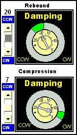
Make + or - changes via the upper buttons for compression and rebound
valve setting to illustrate the different free responses W(t).
Changes between the front and rear measurents via upper left buttons.
A.1) Front Suspension
The graphs showing underdamped second-order and overdamped first-
order transient curves.
The related front trace looks resonable while setting the compression
needle valve to 7ccw and the rebound needle valve to 20ccw.
A.2) Motion W(t) of mass me
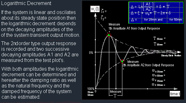
Determine the logarithmic Decrement Δ :
logarithmic decrement Δ [ ] = Ln ( Amplitude A1 / Amplitude A2 )
Coefficient estimation for 25mm Amplitude impulse response :
A1.1 =
[mm]
A1.2 =
[mm]
dΤ 1 =
[sec]
Δ 1 =
[ ]
ζD 1 =
[ ]
ωn 1 =
[Hz]
ω D 1 =
[Hz]
Hydraulic Dashpot Coefficient ß :
With the oil [SAE] depending dashpot coefficient ßoil and measured body mass me
ß [kg/s] = δ [1/s] * 2 * me [kg])
oil flow depending dashpot coefficient
ß [kg/s] = Voil [mm³] / time [s]* ρoil [kg/mm³]
Coefficient estimation for 50mm Amplitude impulse response :
A2.1 =
[mm]
A2.2 =
[mm]
dΤ 2 =
[sec]
Δ 2 =
[ ]
ζD 2 =
[ ]
ωn 2 =
[Hz]
ωD 2 =
[Hz]
Hydraulic Dashpot Coefficient ß :
Estimated 'Damping Factor' δ2 [1/s] = ζD2 [ ] * ωn2 [1/s]
With the oil [SAE] depending dashpot coefficient ßoil and measured body mass me
ß [kg/s] = δ [1/s] * 2 * me [kg])
oil flow depending dashpot coefficient
ß [kg/s] = Voil [mm³] / time [s]* ρoil [kg/mm³]
A.3) Terms of Time-Domain-Output's
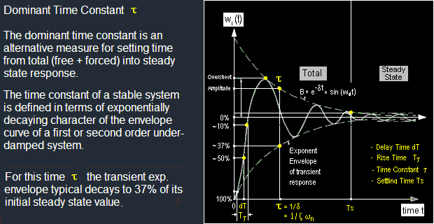
Specify the Over- and Undershoot's
Over- and Undershoots are maximum differences between the transient
amplitudes and the steady state level for a disturbance input. It is a
measure of relative stability and is often represented as a % of the
final value of the steady-state output.
Specify the Delay Time
The Delay Time, interpreted as a time-domain specification, is often
defined as the time required for the system response to a disturbance
input to reach 50 % of its steady state set up level.
Specify the Rise Time
The Rise Time, depends on the system and its adjustments. It defines the
time required for the body mass me to rise from 90 to 10 % of its final
value.
Specify the Settling Time
The settling time is most defined as the time required to reach zero for
the transient part and remain at Steady State Equlibrium Level within a
specified tolerance.
A.4) Set Up Goal for Front Free Response W(t):
W(t) shall have 1 Overswing and 1 X Underswing and reach steady state within approx. 1 second after impulse input.
Measuring Results for Front Set Up
The measurement shows that the optimal underdamped curve with one
overshoot and one underswing corresponds to 7ccw for compression
and 20ccw for rebound needle valve set up's.
Total Free Response Time for 25mm amplitude
For the 25mm compression amplitude input y(t) the total time between
impulse input and reaching the steady state equlibrium level again is
ttotal ~ 0.95s. The time only for the free response W(t) is tW(t)=0.7s .This
free response curve W(t) reaches its first rebound depending amplitude
at ta=0.32s and its second compression depending amplitude at tb=0.53s.
Total Free Response Time for 50mm amplitude
For the 50mm compression amplitude input y(t) the total time between
impulse input and reaching the steady state equlibrium level again is
ttotal ~ 1.05s. The time only for the free response W(t) is tW(t)=0.74s.This
free response curve W(t) reaches its first rebound depending amplitude
at ta=0.31s and its second compression depending amplitude at tb=0.58s.
Note for adjustment and parameterization
With a too low compression damping (pink line) the front will oscillate
several times (m > 2). With a too high compression damping (blue line)
the front will get overdamped. With a too low rebound adjustment the
response curve W(t) will come back too tough to the steady state level.
The yellow response line shows a characteristics to be met for both
amplitudes.
_Re20(23)_Both_Farbe.bmp)
A.5) Actual Front Set Up Öhlins Type FG43 813
Installation dimesion
Spring Type with 260mm free spring lenght
Front Spring Rates
Actual 2 Spring(s) with 2 X 10.5N/mm for both legs
Front Spring Pre-Load adjustment
Note:
- adjustment steps 1mm per turn
- assembly lenght = 2mm
- adjustment range = 2mm .... 12mm
Actual Pre-Load Set Up lenght = 8mm ≡ 6 turns
Damping
SAE oil Types ( 1 centriStroke = 1mm²/s ; 1 Stroke = 10-4m²/s )
Actual oil Type ≡ 19 [cSt] @ 40 [°C]
oil Level respectively Air Cussion
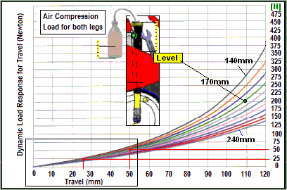
Actual oil Level: 170mm Air Cussion ≡ green line
oil Level for 170mm Air Cussion Spring Curve
Compressed Air for 25mm Fair = 20N ~ 2kg , low influence at 25mm
Compressed Air for 50mm Fair = 50N ~ 5kg , low influence at 50mm
The damping depends on the hydraulic oil flow Q via valves
Hydraulic oil-Flow Qoil [mm³/s] = Avalve [mm²] * Velocityoil [mm/s]
The Hydraulic oil-Velocity Voil [m/s] is obtained by dividing the
oil-Flow Q by the valve opening area A.
The 'Damping Force' is a function of the 'Hydraulic oil Velocity'.
- Fhydraulic = ßoil[kg/s] * velocityoil[m/s] , ß = f(oil Type and Temperature)
Hereby the flow characteristic is represented by the dashpot coefficient ß.
Dynamic's and the characteristic which can be adjusted :
Hydraulic Operating Area within both yellow lines
Max. Hydraulic compression CurveFcompression ~ 0.15KN(15kg)...0.5KN(50kg)..
Max. Hydraulic rebound CurveFrebound ~ 0.30KN(30kg) ... 0.80KN(80kg)..
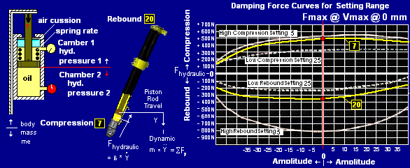
The above figure illustrates the hydraulic force lines Foil for compression
and rebound; however the damping is defined by the hydraulic force
Foil as a function of the oil flow velocity. Hereby the selected valve
opening provides the oil flow quantity into the chamber corresponding
to the piston rod low or high speed travel direction. Needle valves in
the rod for low flow velocities as well as shims as part of the piston
area for high flow velocities. Both dimensions can be changed to meet
needed characteristcs.
A.6) Rear Suspension
The graphs showing overdamped first order transient curves.
The related rear trace looks resonable while setting the compression
needle valve to 11ccw and the rebound needle valve to 35ccw.
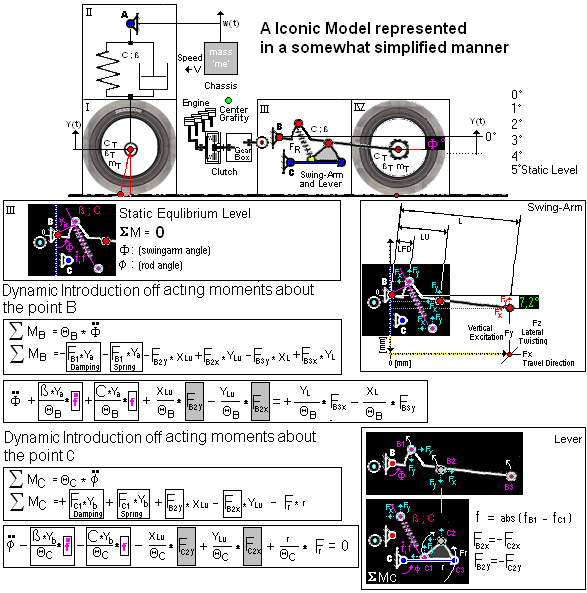
A.7) Primary- and Final- Drive Set Up for Swingarm & Shockabsorber
Shock Absorber Kinematic & Dynamic Ranges
Swingarm Angle α = 5° Absorder Travel Y = 0 mm + 15mm Fspring = 1.4KN ~ 145kg
Swingarm Angle α = 4° Absorder Travel Y = 4 mm + 15mm Fspring = 1.8KN ~ 186kg
Swingarm Angle α = 3° Absorder Travel Y = 8 mm + 15mm Fspring = 2.2KN ~ 228kg
Swingarm Angle α = 2° Absorder Travel Y = 13 mm + 15mm Fspring = 2.6KN ~ 270kg
Swingarm Angle α = 1° Absorder Travel Y = 18 mm + 15mm Fspring = 3.0KN ~ 308kg
Longitudinal Force Pinion Sproket Vertical Travel
[KN]
[mm]
Selected Shock Absorber Coil Spring:
The steady state equlibrium level devides the swingarm travel in a
positive part for compression (~ 2/3) and a negative travel part for
rebound (~ 1/3). This static zero line is adjusted with the coil spring
pre-load setting (rest position for rear body mass me: -5° ~ 15mm ).
The longitudinal force through the rear wheel shaft axle causes a
clockwise (+) moment around the swingarm bearing. The chain force
causes a counter clockwise (-) moment around the swing arm bearing.
Both chain drive and longitudinal moments are summed. If this sum acts
counter clockwise (-) the swing arm will be pulled into the suspension.
Herby the selected coil spring of the shock absorber will be compressed.
With smaller swingarm angles, the coil spring gets more compressed.
If the total sum of moments incl. the compressed shock absorber spring
is acting clockwise this moment (+) will push the tire against the surface.
Which provides grip depending on the actual surface friction.
For a rear input y(t) the transient compression or rebound response w(t)
shall not under- or overswing the steady state equlibrium level a 2nd time
(1th order motion from the rest position expected).
A.8) Set Up Goal for Rear Free Response W(t):
W(t) shall have no Overshoots and reach steady state within approx.
1 second after impulse input.
Measuring Results for Rear Set Up
The measurement shows that the optimal overdamped curve with no
overshoot and no underswing corresponds to 11ccw for compression
and 35ccw for rebound needle valve set up's.
Total Free Response Time for 10mm amplitude
For the 10mm compression amplitude input y(t) the total time between
impulse input and reaching the steady state equlibrium level again is
ttotal ~ 0.45s. The time only for the free response W(t) is tW(t)=0.26s.
Total Free Response Time for 20mm amplitude
For the 20mm compression amplitude input y(t) the total time between
impulse input and reaching the steady state equlibrium level again is
ttotal ~ 0.63s. The time only for the free response W(t) is tW(t)=0.39s.
Note for adjustment and parameterization
The rear shall not oscillate such as the front and must show a 1th order
overdamped free response. The blue line shows a lower rebound damping
effect. The decaying to steady state level becomes faster. The pink line
shows a higher rebound damping effect. Here the decaying to the steady
state equlibrium level becomes slower (settling time shall not be too
slow < 0.8s e.g. running wide effect while cornering). The yellow response
line shows a characteristics to be met for both amplitudes.
A.7) Actual Rear Set Up
Shock Absorbe Öhlins Type 46PRXLS Type S46 Series HO604
Installation dimesion
Absober Mounting Lenght = 311mm which is shortest possible geometric mounting lengh
Spring Type with actual measured 147mm free spring lenght L1 and with 84mm spring block lenght L2
Type 0 1093 36 / yyy L1 311 = Nominal 150mm free spring lenght
Type 0 1091-36 / yyy L1 311 = Nominal 160mm free spring lenght
Type 0 1092-36 / yyy L1 311 = Nominal 170mm free spring lenght
Maximal posible spring compression displacement
Max. Spring Comp. Travel = Free Lenght L1 - Block Lenght L2 ~ 60mm
Rear Spring Rates
Type 0 xxxx 36 / 095 L1 311 Actual 1 X Spring with 95.0N/mm for rear swing arm
Rear Spring Pre-Load adjustment
Actual Pre-Load = 145kg: 147mm-132mm = 15mm compressed ≡ 8 turns
Rear Pre-Load = 174kg : 147mm-129mm = 18mm compressed ≡ 10 turns
Rear Pre-Load = 213kg : 147mm-125mm = 22mm compressed ≡ 12 turns
Damping
The damping depends on the hydraulic oil flow Q via valves
Hydraulic oil-Flow Qoil [mm³/s] = Avalve [mm²] * Velocityoil [mm/s]
The Hydraulic oil-Velocity Voil [m/s] is obtained by dividing the
oil-Flow Q by the valve opening area A.
The 'Damping Force' is a function of the 'Hydraulic oil Velocity'.
- Fhydraulic = ßoil[kg/s] * velocityoil[m/s] , ß = f(oil Type and Temperature)
Hereby the flow characteristic is represented by the dashpot coefficient ß.
Dynamic's and the characteristic which can be adjusted :
Hydraulic Operating Area within both yellow lines
Max. Hydraulic compression CurveFcompression ~ 2.0KN(200kg)...2.3KN(230kg) ...
Max. Hydraulic rebound CurveFrebound ~ 2.0KN(200kg) ... 4.1KN(410kg) ...
The above figure illustrates the hydraulic force lines Foil for compression
and rebound; however the damping is defined by the hydraulic force
Foil as a function of the oil flow velocity. Hereby the selected valve
opening provides the oil flow quantity into the chamber corresponding
to the piston rod low or high speed travel direction. Needle valves in
the rod for low flow velocities as well as shims as part of the piston
area for high flow velocities. Both dimensions can be changed to meet
needed characteristcs. The Nitrogen Gas in the expansion reservoir allows
to keep the oil always under a constant pressure.
B) Control Loop Categories
B.1) Open Control Loops
An Open Loop Control Feature is one in which the control action is
independent of the output response. Their ability to perform accu-
rately is determined by their calibration to obtain a desired system
output. Normaly without problems of instability. Proper performance
must be checked by the user. It is not possible to carry out improve-
ments during real time operation once the system characteristics has
been set. Mostly you find one acceptable set up operation point such
as shown in the test traces.
B.2) Closed Control Loops
A Closed Loop Control Feature is one in which the control action is
dependent of the output signal response while the output signal is
compared with the input signal so that a proper control action can
be formed by a control device HW and SW during real time operation.
The controlled output signal returns back and is algebraically summed
with an required output signal. This error signal is used to command
a specific action such as adjustment and parameterization to obtain an
ideal output signal for the body mass, kinematics of the spring/damper
system used, the road surface pertubations, the overall dynamics of the
vehicle system and special operating maneuvers.
C) Design or Application Objectives
The basic goal of "Functional Design" is to fulfill the performance spec's
in accordance with the functional safety strategies.
External or/and internal disturbances or operating maneuvers affects the
steady state equlibrium Level.
Open loop concepts with manual pre-adjustments or closed loop feedback
control concepts can be applied to reach the desired output value in a
required manner.
Functional release spec' for linear systems may be in form of
Time-Domain-Requirement's in terms of required time responses
(Measure motion W(t) returning to steady state after excitation)
and/or
Frequency-Domain-Requirement's in terms of values related to frequency.
(A transformation technique relating time domain function into a frequency
domain dependening function with the "complex variable S" is the well
known as the "Laplace Transformation" for linear systems)
D) Objective of Analysis
Determination of following system characterisitics:
I) What is the Characteristic Equation W(t) of the total motion ?
II) What is the Transient Motion Part (Free Response of W(t))?
III) What is the Steady State Motion Part (Forced Response of W(t)) ?
IV) What is the Stability or how close is the system to become unstable ?
V) What Functional Safety Strategies are implemented ?
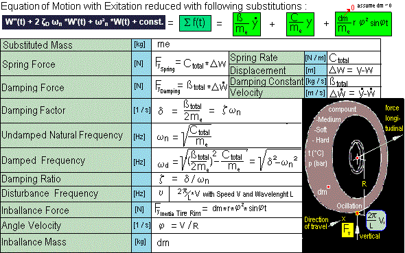
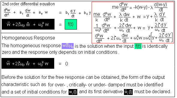
E) Equation W(t) describing the motion of the bodymass me :
E.1) Linear and nonlinear motion
The linear differential equation consists of a sum of linear terms.
d2W / dt2 + 2 ζD ωn * d1W / dt1 + ω²n * d0W / dt0 = ω²n * [ y(t)1+ y(t)2 +...+ y(t)m]
A term consists of a dependent variable W(t) or it's derivatives Wn'(t)
and products and quotients of explicit function's y(t)nm of the independent
variable time t.
In the above equation W(t) is the displacement of the body mass me
- 1th derivative is the 'Velocity' of the body mass me: w'(t) = dW / dt
- 2nd derivative is the 'Acceleration' of the body mass me: w"(t) = d2W / dt2
W"(t) + 2 ζD ωn *W'(t) + ω²n *W(t) = ω²n * y(t)m
∑ ak dkW / dtk = ∑ bk dky / dtk
where W = W(t) is the output and y = y(t) is the input
If all coefficient's ak and bk on both sides of the equation depend only upon
the independent variable time, the system is a 'Linear Differential Equation'
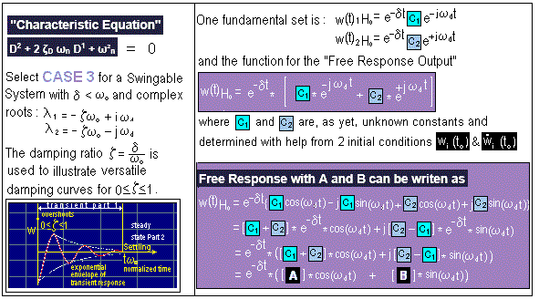
Characteristic equation describing the shape of the free response with
differential operator D and coefficient's ak .
D2 + 2 ζD ωn D1 + ω²n = 0
∑ ak Dk = 0
Linear models which vary with time are describable by linear time-invariant
ordinary differential equations excited by deterministic (not random)
laplace transformable input functions y(t)m.
All physical systems are nonlinear to some extent. No physical system
is exactly linear or vary with time as well as no disturbance input is
completely deterministic. Therefor linear models are approximations and
broad applications and in some cases invalid or inappropriate !
Fortunately, a large percentage of installed systems can be presented by
linear models over a specified operating range.
Note for the concept of linearity
A linear system is a system which has the property that :
If an Input y1(t) produces an output W1(t) and an Input y2(t) produces an Output W2(t)
Then an Input b1 * y1(t) + b2 * y2(t) produces an Output a1 * W1(t) + a2* W2(t)
for all pairs of Input's and all pairs of constant coefficient's.
E.2) Most significant coefficient's ζD and ωn:
The measured curve can be approximated as a 2nd order free response describing the system.
The caracteristic equation D
2 + 2 ζ
D ω
n D
1 + ω²
n = 0 describes the shape of the motion
W(t)
with the 2 solutions of the differential operator D.
Both roots become :
D
1 = - ζ
D ω
n + j * ω
n √(1 - ζ
D²) = δ + j * ω
D
D
2 = - ζ
D ω
n - j * ω
n √(1 - ζ
D²) = δ - j * ω
D
The parameter defining the shape of the curve is the 'Damping Ratio' ζ
D.
Following cases for the variable coefficient 'Damping Ratio' ζ
D :
ζ
D = 0
ζ
D < 0
ζ
D > 1
ζ
D = 1
or ζ
D for an underdamped 2nd order response 0 < ζ
D < 1 which presents the measured underdamped 2nd order physical system.
Where the constant positive coefficient ω
n is called 'Undamped Natural Frequency' of the system.
E.3) Damping Factor
δ is called the 'Damping Factor. δ = ζ
D [ ] * ω
n.
Where 1/ δ is the 'Time Constant τ' of the physical system.
E.4) Damped Natural Frequency ωD
ω
D = ω
n * √(1 - ζ
D²) is called the 'Damped Natural Frequency' of the physical system.
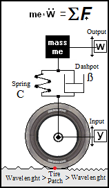
F) Basis Newtons Second Law
The sum of all acting forces to the body mass m
e is related to the
acceleration of the body mass.
m
e * d
2W / dt
2 = ∑ F
Mechanical front system
3 Forces acting simultaneously on the tire contact point from different
directions x, y and z. Measuring the vertical acceleration at the axle has
the advantage, that the interaction between the surface and the tire does
not need to be explicitily known. Assumption that the spring / damper
properties of the tire can be neglected and that the wheel mass is small.
Further there can be a harmonic load excitation as shown with the
inballanced disturbance mass dm.
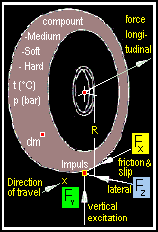
Of particular interest at this test is the case where forces acting toward
y direction
where F
y is the force in y direction, m
e is the body mass, C is the spring
rate, ß
D is the oil depending dashpot coefficient, F
μ is the friction,
and dm is the inballanced mass and W = W(t) is the body mass output
motion and y = y(t) is the axle input motion (road profile).
The iconic model shows a 2nd order differential equation with the significnt coefficient's
W"(t) + 2 ζ
D ω
n *W'(t) + ω²
n *W(t) + const. = ω²
n * [ y'(t)
m + y(t)
m ]
Overview Definitions
F.1) Special motion of the rear swing arm and lever arangement
Here the sum of all acting moments about the mounting point B and the
mounting point C related to the angle acceleration of the inertia are
of interest.
θ
B * d
2φ / dt
2 = ∑ M
B
θ
C * d
2φ / dt
2 = ∑ M
C
F.2) Plot Solution of Motion W(t):
The above plot for Time-Domain Characteristc's for underdamped
2nd Order differential equation should help to visualize the motion.
The plot simply calculates the motion W(t) using the formular's
illustrated next, and plots the graph showing shape of the motion.
The buttons are used to change the shape by parameters in the
system such as changing the Damping Ratio or the Disturbance
Frequency or the Spring Rate or the Weight.
F.3) Determine Solution of Motion W(t):
The total solution for the motion W(t) can be devided into a "Free
Response" and a "Forced Response"

The free response is that part of the total response which approaches
zero as time approaches infinity (transient's). The steady state response
is that part of the total response which does not approaches zero as time
approaches. Steady state disturbances such as ocillating input's e.g. from
the road surface irregularities.
F.4) Determine Free Response with "Characteristic Equation"
F.4.1) Determine Free Response with "Characteristic Equation"
F.4.2) Determine Free Response with "Characteristic Equation"
F.4.3) Determine Free Response with "Characteristic Equation"
F.4.4) Determine Free Response with "Characteristic Equation"
F.5) Find the Steady State Response Part of the motion W(t)
Find the Steady State Response of the constant coefficient ordinary
second order linear differential equation while selecting Representative
Excitation Function(s) for the input f(t) disturbance(s).
F.5.1) Find the Steady State Response Part of the motion W(t) Karl
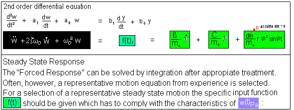
F.5.2) Find the Steady State Response Part of the motion W(t)
F.5.3) Find the Steady State Response Part of the motion W(t)
F.5.4) Find the Steady State Response Part of the motion W(t)
F.5.5) Find the Steady State Response Part of the motion W(t)
F.6) Total Response of the motion W(t)
see above time domain plot W(t)
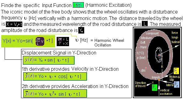
G) Track Surface Irregularities @ steady state operation
G.1) Vertical Acceleration y"(t) = d²y/dt²
Measuring the vertical acceleration at the axle has the advantage, that the
interaction between the surface and the tire does not need to be explicitily
known and that the acceleration value reproduces the dynamic input quite.
well. The vertical acceleration can be specially measured with fixed tire
properties and fixed suspension properties as well as a fixed configuration
of the system at certain speeds. Double integration leads then to a
kinematic disturbance input value y(t) of the road surface which can be
used to optimize the output motions W(t) of the body mass.
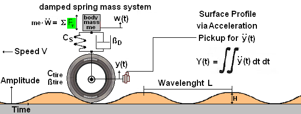
The figure shows a sinusoidal surface profile with a wavelenght L and its
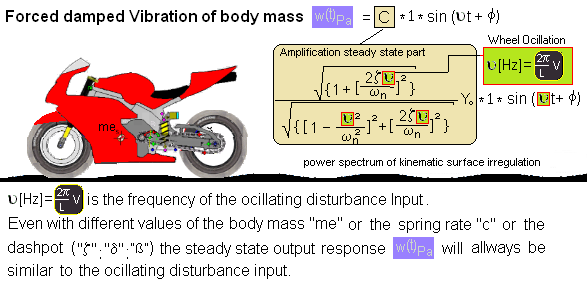
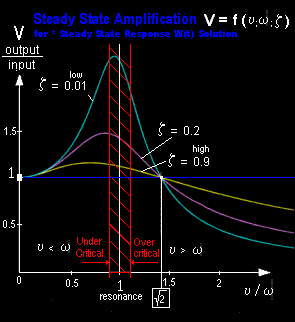
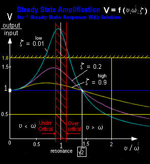
Height H. The wheel will ocillate vertically with y(t) depending on ν [Hz].
Hereby the disturbance frequency ν depends on the wavelengh L and the
vehicle speed V km per hour. If the disturbance frequency ν f(V,L) is close
to natural frequency ω
n of the system, and if the system is only lightly
damped ζ
D → small, → huge amplitudes w(t) of the body mass m
e may
occure (→ Resonance).
Solved Suspension Problem 1:
At what speed V does the maximum amplification of the body mass m
e
occurs, and what is the corresponding resonance amplitude under the
circumstances of an ocillating disturbance υ=f(V;L) and low damping
ratio ζ
D = δ/ω
n ?
Natural Frequency ωn Damping Coefficient ζ
ω
n =
Hz
ζ
D =
Wavelenght L Roughness Height H
L =
m
H =
cm
Vresonance =
km/h
wmax = ½H/ζ =
cm @ ζ =
With resonance Speed at 'Low Damping conditions', the suspension system
is making the vibration worst. Hereby the vibration amplitude w(t)
max of the
body mass m
e will be greater than the surface wave height H.
The behaviour becomes better if a higher damping ζ
Dwill be realized or a
natural frequency ω
nof the system allows to operate the system above the
resonance pole '1' @ ν > ω or @ ν ⁄ω > √2
see following diagram with pole @ 1 = ν/ω
n
Solved Suspension Problem 2:
Under the circumstances of a ocillating wheel disturbance υ(V;L) the
vibration amplitude w(t) of a body mass m
e should not exceed a max
value W
max for all operation speed's ?
Max. Amplification Wmax for all Speed's Irregulation Height
W
max ≤
mm
H
disturbance ≤
mm
Select a necessary damping coefficient ζ
D for an amplification A:
Max amplification factor
A =
[mm]
/
[mm]
=
[ ]
The diagram illustrates that with a damping coefficient ζ
D greater than 0.2
the amplification will not exceed
[ ]
To guarantee that
mm
is kept for all operation speeds following damping
ratio for this ocillating wheel case is adjusted:
ζ ≥
[ ]
Observe in the amplification diagram for steady state that with this damping
coefficient the required amplification factor will not be exceeded.
Solved Suspension Problem 3:
Under the circumstances of a ocillating wheel disturbance υ(V;L) the
amplitude w(t) of the body mass m
e shall be limited at a certain
operation speed V ?
Speed V Max. Amplification for this Speed
V =
km/h
W
V ≤
mm
The disturbance frequency at
V =
km/h is
υ =
Hz
Amplification factor
A =
mm
/
mm
=
@ υ =
Hz
Assure the characteristics for an amplification factor
> ω / υ
Spring stiffness C = ω² * me =
N/mm
Determine the natural frequency ω
n <
* υ
disturbance
ω =
Hz
υ =
Hz
Amplification =
Freq-Ratio υ / ω >
For this operation speed
V =
km/h
it can be observed that the
max amplitude
W
V ≤
mm
can only be kept with an damping ratio
ζ < 0.2 .
Solved Suspension Problem 4:
Determine the optimal spring stiffness C [N/mm] and the dashpot coefficient
ß [kg/s] for the above disturbance case :
Body Mass me
me =
kg
With Natural Frequency
ωn =
Hz
and body mass me =
kg
the springrate for 2 Springs becomes :
C =
N/mm
dashpot coefficient ß = 2* ζD*√me*C
With ζD =
body mass me =
kg
Spring rate C = ω² * me =
N/mm
For this case the required dashpot coefficient becomes :
ß =
kg/s
Solved Suspension Problem 5:
Declare the Damping
The loading pressure Δp [N/mm²] is the pressure difference between rebound
chamber and the compression chamber. This pressure-difference Δp [N/mm²]
acts on the piston area A [mm²] and generates the hydraulic force F [N].
Hydraulic Force F = Δpoil * Apiston
Valves must deliver a volume of oil [mm³] corresponding to the piston rod
travel y [mm].
Hydraulic oil Volume V [mm³] :
Voil = Avalve * Ytravel
Accociated oil Flow Qoil [mm³/s] :
The hydraulic oil flow Qoil through valves depends on the the valve opening
area and the valve resistance.
Qoil = Voil / time = Avalve * Ytravel / time
Accociated with oil Viscosity ν [mm²/s] :
SAE 2.5W: @ 40°C 18mm²/s @ 100°C 4mm²/s
SAE 5W: @ 40°C 23.3mm²/s @ 100°C 4.8mm²/s
SAE 10W: @ 40°C 45.4mm²/s @ 100°C 7.6mm²/s
Hydraulic oil Flow Q = Avalve * Velocityoil
Accociated oil Density ρ [kg/mm³]
SAE 2.5W: @ 15°C 0.826g/cm³
SAE 5W: @ 15°C 0.829g/cm³
SAE 10W: @ 15°C 0.838g/cm³
Dashpot Coefficient ß [kg/s] :
ßoil = Voil / time * ρoil = Avalve * Velocityoil * ρoil =
kg/s
Damping Force Foil [N] :
The damping is defined by the hydraulic oil force Foil as a function
of the oil velocity. As faster the absorber has to operate as higher the response
of the actual damping force. Hereby the damping characteristic depends on the
dashpot coefficient ßoil.
Foil = ßoil * Velocityoil =
kg/s * { Low-Velocityoil ... High-Velocityoil } [m/s]
Low oil Speed's and High oil Speed's :
Needle valves in the rod for low oil flow velocities as well as shims
as part of the piston area for high oil flow velocities are provided
for the hydraulic flow.
With low operation frequencies the oil can pass through the needle
valve geometry into the compression chamber or rebound chamber.
With high operation frequencies the oil can pass through the shim's
configuration located within the piston into the compression chamber
or rebound chamber.
H) Terms of Stability
The output response is strongly dependent on the
- properties of the " system " and " adjustments "
and the
- excitation frequency " ν " of the road disturbances.
For this type of test @ 0 km/h (standing tire) the output characteristic
for all possible valve settings have been stable (responses exponentially
decaying to the steady state
Satisfactory steady state responses can be determined and adjusted according
the power spectrum of the road surface (roughness wavelenght and amplitudes).
If the system is linear the steady state response will have the same
frequency as that of the disturbance inputs ν [Hz].
The system will have to respond satisfactorily and well damped if operated
to close to natural frequency of the system (Resonance).
Typically the magnitude ratio V [input y(t) / output W(t)] of the system
shall not be closer than 15% to 20% to the resonance pol.
The type of poles which are the roots δ + j * ωD and δ - j * ωD of the
characteristic equation D2 + 2 ζD ωn D1 + ω²n = 0 can represent a stable
or not desired marginally stable or not desired unstable W(t) response.
© Last Up Date March. 25, 2019

 "Suspension Set Up (Digital Learning)"